Geospatial data come in two GIS ready formats, raster and vector. Raster data has a pixel based structure, composed of rows and columns for storing values. Raster formats are used to represent continuous data for example images or surfaces. Examples of raster data in common use in the heritage sector include Ordnance Survey historic maps, aerial photographs and lidar derived surface models.
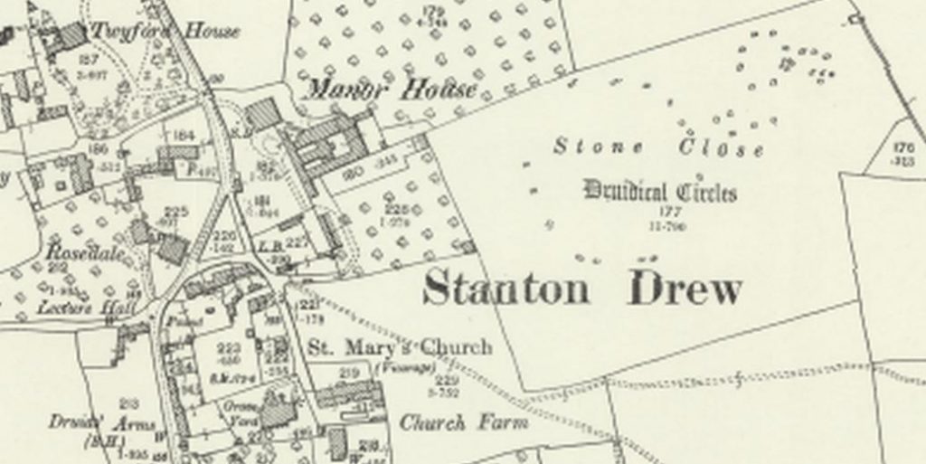
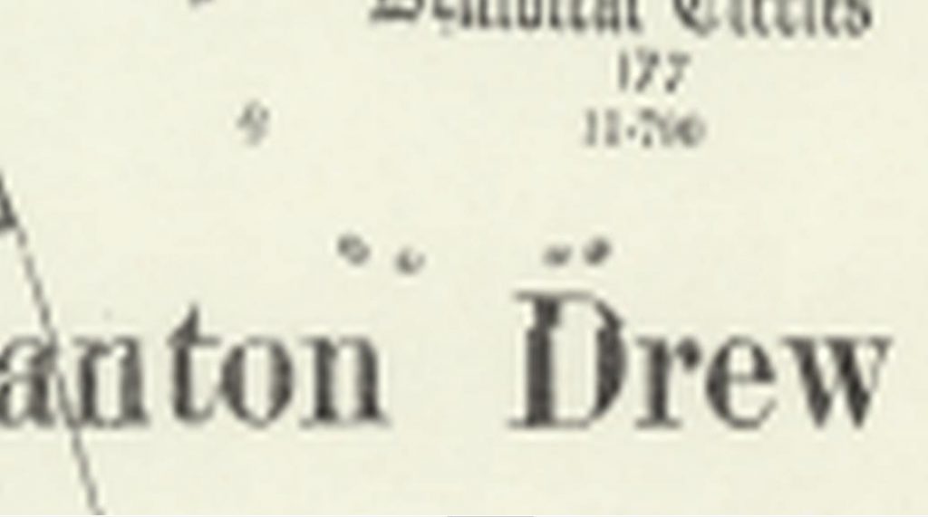
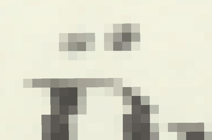
Raster data has a fixed resolution, i.e each pixel (sometimes referred to as a cell) represents a distance on the ground. This means that as you zoom into a raster layer it becomes increasingly pixelated. Raster data are therefore only usable at certain scale ranges.
In Workshop 1 we will look at setting up a QGIS project and adding raster data.
A note on scale
The scale of a map is represented as a ratio of the distance on the map to the distance on the ground. So for a scale of 1:10,000 1cm on the map represents 100m (10,000cm) in reality.
You’ll probably have heard of the common scales used by the Ordnance Survey for their paper maps – 1:2500, 1:25000, 1:50000 and 1:25000. The lower numbers are known as “large scale maps”, and the higher numbers as “low scale”. You can read more about this on the OS website.
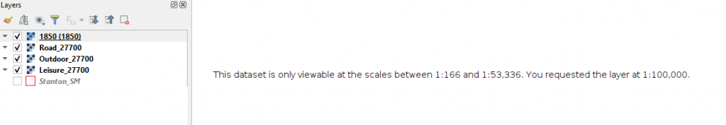
In a GIS scales can be set to any value but as we have seen raster data still display best at particular scales. For raster layers being served over the web this is sometimes controlled via scale dependent rendering where they will only be visible if the project scale is within a certain range (which might lead to messages like the one below).
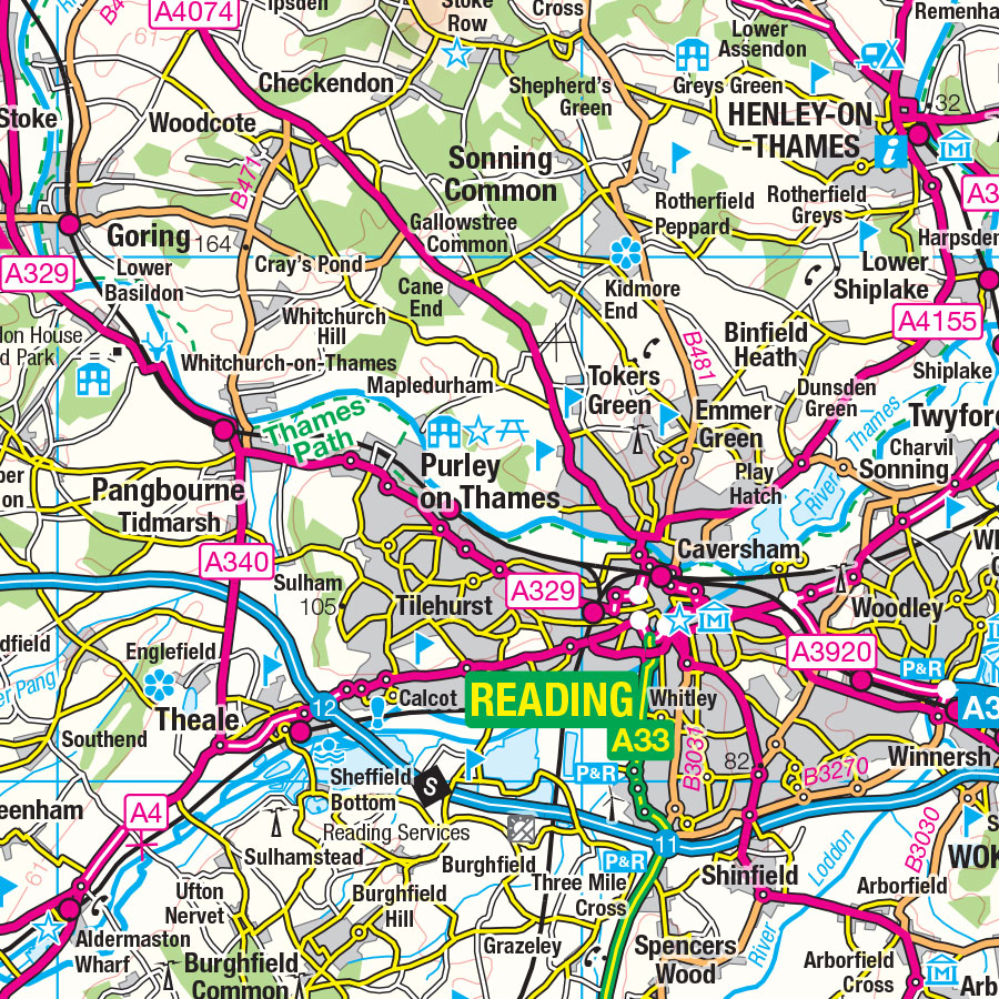
1:250 000 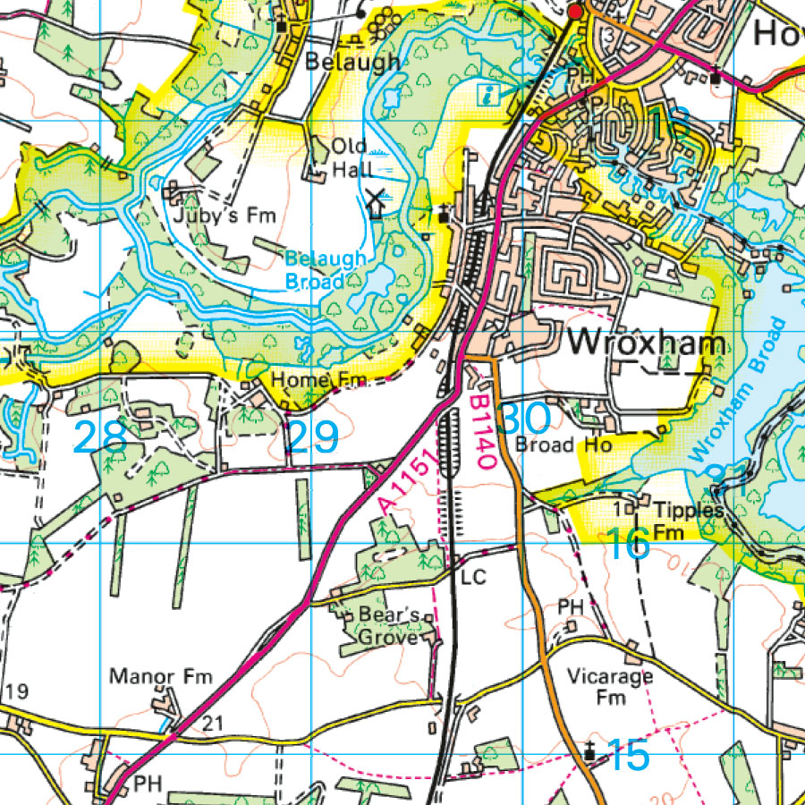
1:50 000 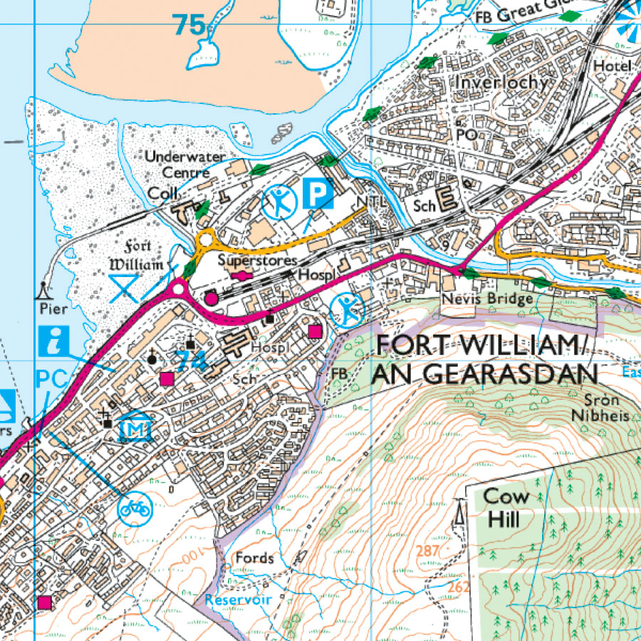
1:25 000 
1:1250